How to Calculate Labour Savings and Payback Period for Factory Automation

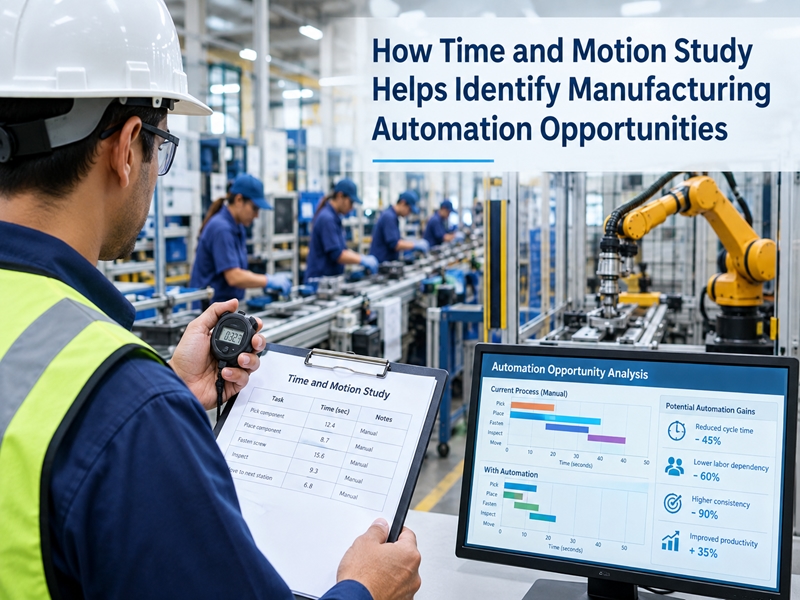
Factory automation can reduce repetitive manual work, improve production consistency and increase manufacturing capacity. However, installing a robot, automated assembly station or packaging system does not automatically translate into lower operating costs. The financial benefit depends on how the equipment changes actual labour requirements, production output, quality performance and ongoing operating expenses.

For manufacturers, the key question is not simply how much faster a machine can operate. It is whether the improvement creates measurable financial value that justifies the investment.

A time-and-motion study for factory automation provides the foundation for answering this question. By measuring operator activities, cycle times, waiting periods and machine utilisation before automation, manufacturers can estimate achievable labour savings and calculate a realistic payback period.

This guide explains the measurement process, essential formulas, a worked manufacturing example and the factors that determine whether an automation project makes financial sense.

Why Time-and-Motion Studies Matter Before Automation

A factory may identify a repetitive operation as a suitable automation candidate because an operator spends considerable time loading components, positioning materials or performing routine assembly. Yet the time spent on that task alone does not establish how many employees the automation system will replace or how much money the business will save.

A time-and-motion study examines the complete production cycle to understand where labour is used and which activities can genuinely be removed, combined or reassigned.

The assessment should establish:

• Manual task time: Time spent handling materials, assembling components, inspecting products and performing repetitive operations.

• Machine cycle time: Time required for equipment to complete its operating sequence, including relevant automatic and idle periods.

• Operator waiting time: Periods when employees wait for machines, materials, instructions or preceding operations.

• Production interruptions: Delays caused by changeovers, equipment failures, material shortages and quality problems.

• Workload distribution: How activities are divided between operators and whether one person can supervise multiple machines safely.

• Post-automation requirements: Remaining duties such as replenishment, inspection, maintenance coordination and process monitoring.

These observations help engineers distinguish between work that disappears, work that shifts to another activity and time that becomes available without producing an immediate payroll reduction.

For example, automating a 30-second assembly task may release significant operator capacity across a high-volume production line. However, if the operator must continue performing other essential tasks, the labour saving may be better expressed as additional available capacity rather than an eliminated position.

Step 1: Establish the Current Labour and Production Baseline

Before calculating savings, measure how the existing operation performs under representative production conditions. Use repeated observations across relevant shifts, product variants and operating conditions rather than relying on a single unusually fast cycle.

Calculate labour hours per unit

The basic formula is:

Suppose a production line has eight operators working eight hours each during a shift and produces 800 acceptable units.

Total direct labour time is:

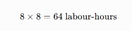
Therefore:

The baseline is 0.08 labour-hours, or 4.8 labour-minutes, per good unit.

This metric helps compare the current process with the proposed automated operation. Use consistent production periods and exclude defective units from the good-output denominator.

Measure the complete work cycle

Break the operation into measurable elements, such as component loading, machine operation, unloading, inspection and transfer to the next workstation.

Record which tasks occur sequentially and which overlap. This distinction is essential because machine operating time and operator working time are not always additive.

The resulting operator-machine chart should show the current work sequence, the time required for each activity and opportunities for combining tasks or assigning one operator to several machines.

Step 2: Calculate the Annual Labour Cost

Labour savings should be calculated using the fully loaded cost of employment rather than basic wages alone.

Include relevant costs such as:

• Annual wages and salaries.

• Employer contributions and employment-related benefits.

• Shift allowances and recurring incentives.

• Other recurring employment costs that will genuinely be avoided.

For a simplified calculation, assume one production employee costs the manufacturer ₹4,20,000 annually, including relevant employment costs.

If automation enables the business to eliminate two positions, the potential annual gross labour saving is:

The estimated gross saving is ₹8.4 lakh per year.

However, this calculation is valid only if both positions can actually be eliminated or their costs avoided. If existing employees are reassigned to other activities, their salaries remain an expense. In that case, the business may gain productive capacity without achieving an equivalent reduction in payroll.

Manufacturers should therefore classify projected labour benefits as:

• Direct cost savings: Employment expenditure that will actually be removed.

• Avoided future costs: Additional hiring that would otherwise be necessary as production grows.

• Redeployed capacity: Existing labour time made available for other productive activities.

• Overtime savings: Additional labour expenditure avoided by reducing overtime requirements.

Keeping these categories separate prevents inflated automation business cases.

Step 3: Calculate the Total Cost of Automation

The purchase price of the machine is only one part of the investment. The calculation should include the costs required to install, integrate and operate the system.

The total installed cost becomes the initial investment used in the payback calculation.

Recurring maintenance, energy, consumables, software subscriptions and additional technical support should generally be recorded as ongoing operating costs rather than added indiscriminately to the initial investment.

This distinction makes the financial model easier to audit and update when actual project costs become available.

Step 4: Calculate Annual Net Financial Benefits

Labour savings alone may not capture the complete value of automation. A system may also reduce scrap, lower overtime expenditure or increase saleable production.

The following formula provides a practical starting point:

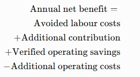
Additional contribution refers to the financial contribution from extra products actually sold, after accounting for their incremental production and selling costs. It should not be confused with gross sales revenue.

Consider these illustrative annual estimates:

These figures illustrate the calculation method; they are not industry averages or guaranteed savings.

Care is needed to avoid double-counting. For example, if additional output is possible because existing employees are redeployed, do not also count those same employees as eliminated positions unless the staffing assumptions genuinely support both benefits.

Step 5: Calculate the Factory Automation Payback Period

The simple payback period estimates how long the annual net financial benefit takes to recover the initial investment.

Suppose the automation project requires ₹52 lakh in total installed investment and is expected to generate ₹14.2 lakh in annual net financial benefits.

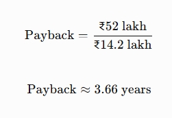
The estimated simple payback is approximately 44 months.

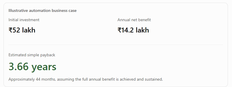
Approximately 44 months, assuming the full annual benefit is achieved and sustained.

This result is useful for preliminary evaluation, but it is not a complete investment appraisal. Simple payback does not account for the time value of money, cash flows after the payback date or changes in annual performance.

For major capital investments, manufacturers should also consider net present value (NPV), internal rate of return (IRR), equipment life, taxes and the timing of implementation costs.

Step 6: Test Whether the Expected Savings Are Achievable

A financial calculation is only as reliable as its assumptions. Time-and-motion findings should be translated into a realistic post-automation staffing plan before labour savings are approved.

For example, suppose manual handling takes 50 seconds per unit before automation and 15 seconds afterwards. At 1,000 units per shift, the reduction in manual task time is:

The operation releases approximately 9.72 hours of manual task time per shift.

That does not automatically mean 1.22 employees can be removed. The released time may be distributed across several operators, overlap with other duties or be needed for material replenishment, inspection and machine supervision.

A post-automation operator-machine analysis should establish the actual staffing requirement.

Factors that can change the payback period

• Equipment utilisation: Insufficient production demand can leave expensive equipment underused.

• Machine reliability: Breakdowns and maintenance interruptions reduce realised output.

• Product variation: Frequent changeovers and different component specifications may limit savings.

• Production bottlenecks: Faster operation at one station may simply transfer the constraint downstream.

• Quality performance: Scrap and rework can offset expected benefits if the new process is not properly validated.

• Staffing arrangements: Redeployment, attrition and future hiring plans determine whether labour benefits become financial savings.

• Commissioning delays: Training and production ramp-up can postpone the start of expected benefits.

A useful practice is to prepare lower-benefit, base-case and higher-benefit scenarios. Calculate payback separately for each scenario rather than presenting one forecast as certain.

Step 7: Avoid Common Automation Investment Mistakes

Manufacturers can improve decision quality by addressing several recurring weaknesses in automation business cases.

1. Counting released time as eliminated labour: A reduction in task duration does not guarantee a reduction in payroll. Confirm the revised staffing plan.

2. Ignoring integration expenses: Excluding tooling, installation, safety systems and commissioning can understate investment.

3. Using theoretical machine speed: Rated cycle time does not necessarily represent actual good output under normal factory conditions.

4. Overestimating incremental sales: Additional production creates financial value only when the products can be sold at an adequate contribution margin.

5. Ignoring ongoing expenses: Maintenance, spare parts, energy and technical support can materially reduce annual benefits.

6. Using payback as the only decision metric: Two projects with similar payback periods can have different useful lives, risks and long-term cash flows. NPV and IRR provide additional perspectives.

These checks help ensure the business case reflects the complete production system rather than the isolated performance of a machine.

How IMARC Engineering Can Help

IMARC Engineering can support manufacturers evaluating automation through time-and-motion studies, manufacturing productivity assessments and automation feasibility analysis, subject to the agreed project scope. The assessment can examine current work cycles, operator utilisation, production bottlenecks and potential staffing changes before investment. By comparing existing and proposed processes, manufacturers can develop a cost model covering equipment, implementation, labour requirements and ongoing operating expenses. This provides a structured basis for evaluating projected savings, payback assumptions and operational risks before committing capital to automation.

Speak With An Expert: https://www.imarcengineering.com/contact?service=time-and-motion-studies

Conclusion

Calculating labour savings and automation payback requires more than comparing machine prices with current wages. Manufacturers must establish a reliable baseline, measure manual work, determine achievable staffing changes, include implementation and operating costs, and validate benefits against actual production requirements. Time-and-motion studies connect these operational findings to financial calculations, helping decision-makers distinguish genuine cost reductions from released capacity. Combining measured data with scenario analysis, payback calculations and longer-term investment evaluation creates a more defensible basis for deciding whether factory automation is financially justified.

Contact Us:

IMARC Engineering

Phone: +91-120-433-0800

Email: sales@imarcengineering.com

India: C-130, Sector 2, Noida, Uttar Pradesh 201301

LinkedIn: https://www.linkedin.com/showcase/imarc-engineering/